Handling Imbalanced Datasets with SMOTE in Python

Introduction: balanced and imbalanced datasets

Close your eyes. Now imagine a perfect data world. What do you see? What do you wish to see? Exactly, me too. A flawlessly balanced dataset. A collection of data whose labels form a magnificent 1:1 ratio: 50% of this, 50% of that; not a bit to the left, nor a bit to the right. Just perfectly balanced, as all things should be. Now open your eyes, and come back to the real world.

The opposite of a pure balanced dataset is a highly imbalanced dataset, and unfortunately for us, these are quite common. An imbalanced dataset is a dataset where the number of data points per class differs drastically, resulting in a heavily biased machine learning model that won’t be able to learn the minority class. When this imbalanced ratio is not so heavily skewed toward one class, such dataset is not that horrible, since many machine learning models can handle them. 

Nevertheless, there are some extreme cases in which the class ratio is just wrong, for example, a dataset where 95% of the labels belong to class A, while the remaining 5% fall under class B– a ratio not so rare in use cases such as fraud detection. In these extreme cases, the ideal course of action would be to collect more data. 

However, this is typically not feasible; in fact, it’s costly, time-consuming and in most cases, impossible. Luckily for us, there’s an alternative known as oversampling. Oversampling involves using the data we currently have to create more of it. 

What is data oversampling?

Data oversampling is a technique applied to generate data in such a way that it resembles the underlying distribution of the real data. In this article, I explain how we can use an oversampling technique called Synthetic Minority Over-Sampling Technique or SMOTE to balance out our dataset.

What is SMOTE?

SMOTE is an oversampling algorithm that relies on the concept of nearest neighbors to create its synthetic data. Proposed back in 2002 by Chawla et. al., SMOTE has become one of the most popular algorithms for oversampling. 

The simplest case of oversampling is simply called oversampling or upsampling, meaning a method used to duplicate randomly selected data observations from the outnumbered class. 

Oversampling’s purpose is for us to feel confident the data we generate are real examples of already existing data. This inherently comes with the issue of creating more of the same data we currently have, without adding any diversity to our dataset, and producing effects such as overfitting. 

Hence, if overfitting affects our training due to randomly generated, upsampled data– or if plain oversampling is not suitable for the task at hand– we could resort to another, smarter oversampling technique known as synthetic data generation.

Synthetic data is intelligently generated artificial data that resembles the shape or values of the data it is intended to enhance. Instead of merely making new examples by copying the data we already have (as explained in the last paragraph), a synthetic data generator creates data that is similar to the existing one. Creating synthetic data is where SMOTE shines.

How does SMOTE work?

To show how SMOTE works, suppose we have an imbalanced two-dimensional dataset, such as the one in the next image, and we want to use SMOTE to create new data points.

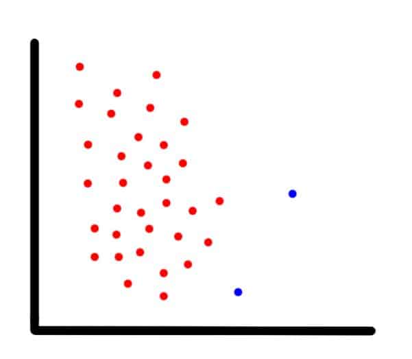
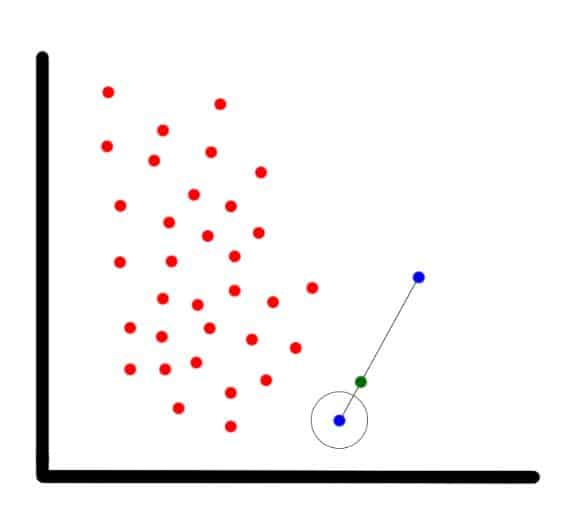
For each observation that belongs to the under-represented class, the algorithm gets its K-nearest-neighbors and synthesizes a new instance of the minority label at a random location in the line between the current observation and its nearest neighbor. 

In our example (shown in the next image), the blue encircled dot is the current observation, the blue non-encircled dot is its nearest neighbor, and the green dot is the synthetic one.

SMOTE tutorial using imbalanced-learn

In this tutorial, I explain how to balance an imbalanced dataset using the package imbalanced-learn. 

First, I create a perfectly balanced dataset and train a machine learning model with it which I’ll call our “base model”. Then, I’ll unbalance the dataset and train a second system which I’ll call an “imbalanced model.”

Finally, I’ll use SMOTE to balance out the dataset, followed by fitting a third model with it which I’ll name the “SMOTE’d” model. By training a new model at each step, We’ll be able to better understand how an imbalanced dataset can affect a machine learning system.

Base model

Example code for this article may be found at the Kite Blog repository.

For the initial task, I’ll fit a support-vector machine (SVM) model using a created, perfectly balanced dataset. I chose this kind of model because of how easy it is to visualize and understand its decision boundary, namely, the hyperplane that separates one class from the other.

To generate a balanced dataset, I’ll use scikit-learn’s make_classification function which creates n clusters of normally distributed points suitable for a classification problem. 

My fake dataset consists of 700 sample points, two features, and two classes. To make sure each class is one blob of data, I’ll set the parameter n_clusters_per_class to 1. 

To simplify it, I’ll remove the redundant features and set the number of informative features to 2. Lastly, I’ll useflip_y=0.06 to reduce the amount of noise. 

The following piece of code shows how we can create our fake dataset and plot it using Python’s Matplotlib.

import matplotlib.pyplot as plt
import pandas as pd

from sklearn.datasets import make_classification
from imblearn.datasets import make_imbalance

# for reproducibility purposes
seed = 100

# create balanced dataset
X1, Y1 = make_classification(n_samples=700, n_features=2, n_redundant=0,
                            n_informative=2, n_clusters_per_class=1,
                            class_sep=1.0, flip_y=0.06, random_state=seed)

plt.title('Balanced dataset')
plt.xlabel('x')
plt.ylabel('y')
plt.scatter(X1[:, 0], X1[:, 1], marker='o', c=Y1,
           s=25, edgecolor='k', cmap=plt.cm.coolwarm)
plt.show()
# concatenate the features and labels into one dataframe
df = pd.concat([pd.DataFrame(X1), pd.DataFrame(Y1)], axis=1)
df.columns = ['feature_1', 'feature_2', 'label']
# save the dataset because we'll use it later
df.to_csv('df_base.csv', index=False, encoding='utf-8')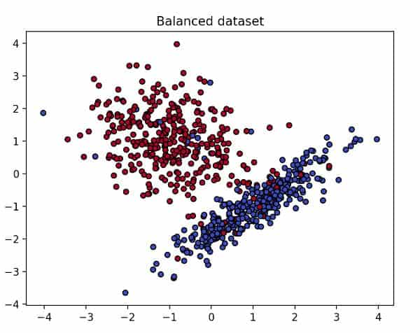

As you can see in the previous image, our balanced dataset looks tidy and well defined. So, if we fit an SVM model with this data (code below), how will the decision boundary look?

Since we’ll be training several models and visualizing their hyperplanes, I wrote two functions that will be reused several times throughout the tutorial. The first one, train_SVM, is for fitting the SVM model, and it takes the dataset as a parameter. 

The second function, plot_svm_boundary, plots the decision boundary of the SVM model. Its parameters also include the dataset and the caption of the plot. 

These are the functions:

import matplotlib.pyplot as plt
import numpy as np
import pandas as pd
from sklearn.svm import SVC


def train_SVM(df):
   # select the feature columns
   X = df.loc[:, df.columns != 'label']
   # select the label column
   y = df.label

   # train an SVM with linear kernel
   clf = SVC(kernel='linear')
   clf.fit(X, y)

   return clf


def plot_svm_boundary(clf, df, title):
   fig, ax = plt.subplots()
   X0, X1 = df.iloc[:, 0], df.iloc[:, 1]

   x_min, x_max = X0.min() - 1, X0.max() + 1
   y_min, y_max = X1.min() - 1, X1.max() + 1
   xx, yy = np.meshgrid(np.arange(x_min, x_max, 0.02), np.arange(y_min, y_max, 0.02))

   Z = clf.predict(np.c_[xx.ravel(), yy.ravel()])
   Z = Z.reshape(xx.shape)
   out = ax.contourf(xx, yy, Z, cmap=plt.cm.coolwarm, alpha=0.8)

   ax.scatter(X0, X1, c=df.label, cmap=plt.cm.coolwarm, s=20, edgecolors='k')
   ax.set_ylabel('y')
   ax.set_xlabel('x')
   ax.set_title(title)
   plt.show()

To fit and plot the model, do the following:

df = pd.read_csv('df_base.csv', encoding='utf-8', engine='python')
clf = train_SVM(df)
plot_svm_boundary(clf, df, 'Decision Boundary of SVM trained with a balanced dataset')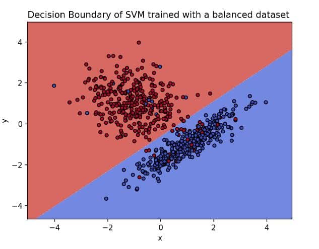

Blue dots on the blue side and red dots on the red side means that the model was able to find a function that separates the classes

The image above presents the hyperplane of the base model. On it, we can observe how clear the separation between our classes is. However, what would happen if we imbalance our dataset? How would the decision boundary look? Before doing so, let’s imbalance the dataset by calling the function make_imbalance from the package, imbalanced-learn.

Imbalanced model

While calling make_imbalance, I manually set my sampling strategy to have finer control of how I want to distribute the data; in this case, I want 340 points to belong to class 0 (red), and 10 points in class 1 (blue):

X_res, y_res = make_imbalance(X1, Y1, sampling_strategy={0: 340, 1: 10}, random_state=seed)
plt.title('Imbalanced dataset')
plt.xlabel('x')
plt.ylabel('y')
plt.scatter(X_res[:, 0], X_res[:, 1], marker='o', c=y_res,
           s=25, edgecolor='k', cmap=plt.cm.coolwarm)
plt.show()


df = pd.concat([pd.DataFrame(X_res), pd.DataFrame(y_res)], axis=1)
df.columns = ['feature_1', 'feature_2', 'label']
df.to_csv('df_imbalanced.csv', index=False, encoding='utf-8')

This is how the imbalanced dataset looks:

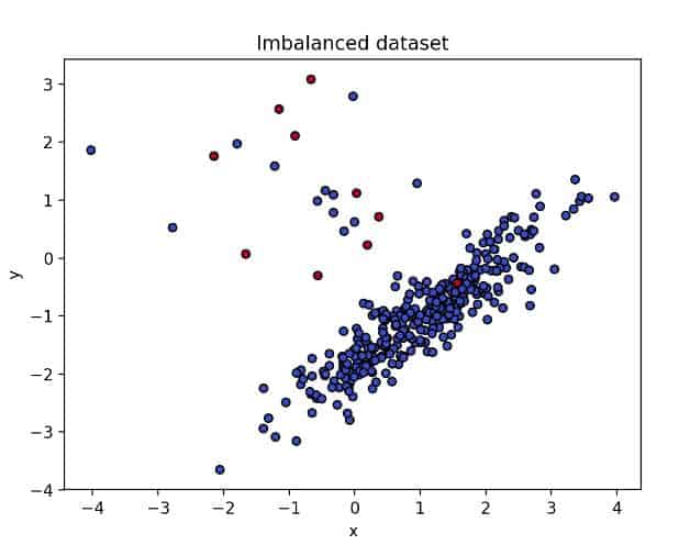
Quite different, right? Now that we have a very, very, imbalanced dataset, let’s train a second SVM and compare the decision boundary.

df = pd.read_csv('df_imbalanced.csv', encoding='utf-8', engine='python')
clf = train_SVM(df)
plot_svm_boundary(clf, df, 'Decision Boundary of SVM trained with an imbalanced dataset')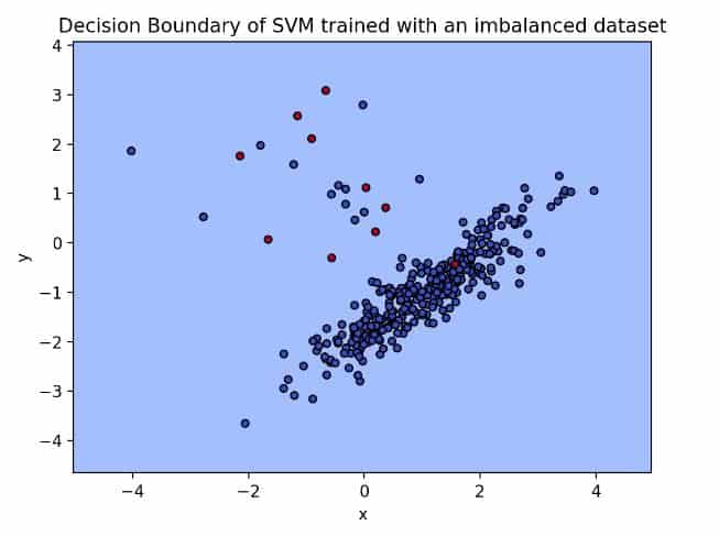

No decision boundary at all. By creating an over-the-top imbalanced dataset, we were able to fit an SVM that shows no decision boundary. In other words, the algorithm was not able to learn from its minority data because its decision function sided with the class that has the larger number of samples.

SMOTE’d model

Now comes the exciting part: suppose that you face a situation like this in a real problem, and sadly, you are not able to obtain more real data. Enter synthetic data, and SMOTE. 

Creating a SMOTE’d dataset using imbalanced-learn is a straightforward process. Firstly, like make_imbalance, we need to specify the sampling strategy, which in this case I left to auto to let the algorithm resample the complete training dataset, except for the minority class. Then, we define our k neighbors, which in this case is 1. The next piece of code shows how to enhance the previous, imbalanced dataset using SMOTE.

import pandas as pd
import matplotlib.pyplot as plt

from imblearn.over_sampling import SMOTE

# for reproducibility purposes
seed = 100
# SMOTE number of neighbors
k = 1

df = pd.read_csv('df_imbalanced.csv', encoding='utf-8', engine='python')
# make a new df made of all the columns, except the target class
X = df.loc[:, df.columns != 'label']
y = df.label
sm = SMOTE(sampling_strategy='auto', k_neighbors=k, random_state=seed)
X_res, y_res = sm.fit_resample(X, y)

plt.title('Dataset balanced with synthetic or SMOTE'd data ({} neighbors)'.format(k))
plt.xlabel('x')
plt.ylabel('y')
plt.scatter(X_res[:, 0], X_res[:, 1], marker='o', c=y_res,
           s=25, edgecolor='k', cmap=plt.cm.coolwarm)
plt.show()

df = pd.concat([pd.DataFrame(X_res), pd.DataFrame(y_res)], axis=1)
# rename the columns
df.columns = ['feature_1', 'feature_2', 'label']
df.to_csv('df_smoted.csv', index=False, encoding='utf-8')

The following image displays the resulting dataset.

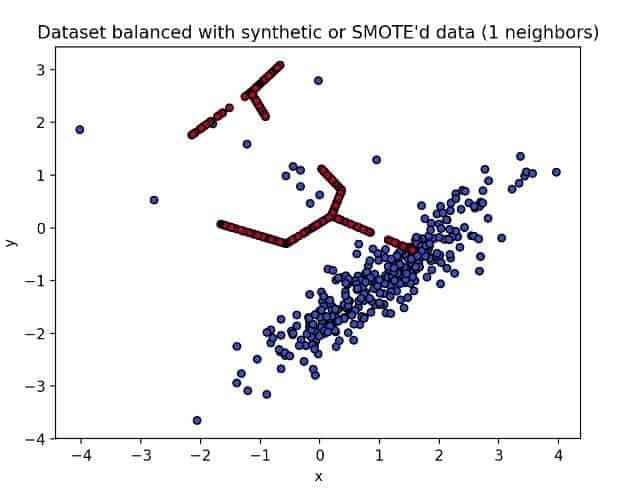
New data! In this image, we can appreciate a more complete dataset compared to the imbalanced one. However, something seems off. It looks like the algorithm generated the new synthetic points in such a way that it resembles a line. 

This line, upon further inspection, appears to be connecting the dots of the imbalanced data points. The explanation behind this phenomenon is that we are using k=1. Setting the number of neighbors to 1 implies that during each iteration of SMOTE, the algorithm creates artificial data between the point it’s currently examining and the one that it’s closer to (as we saw in the first example). 

Thus, since the connection between two points is a line, our final dataset looks like a line that was created by connecting all the dots.

If we increase k to 2, we can see how the connectivity across points extends.

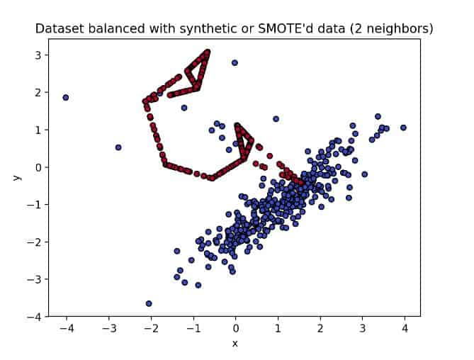
With k=8 we can observe a more vibrant, spherical, and classic looking dataset. 

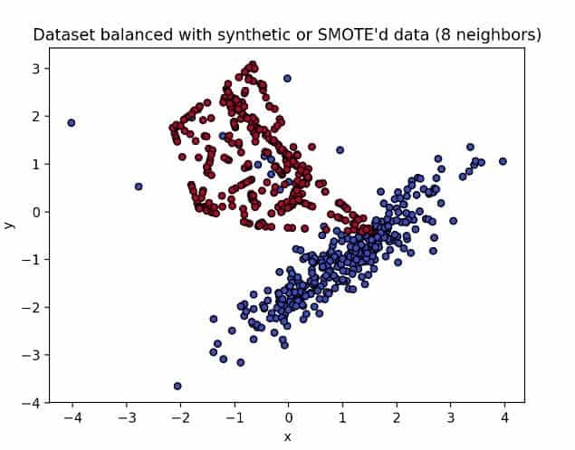
If we compare this dataset with the original one, we can see that the main difference is how tightly self-contained the new data are. 

The compactness of the data might have happened because, unlike the original data, the red class of this SMOTE’d dataset doesn’t have much noise nor many outliers (because we removed them during the creation of the imbalanced dataset). As a result, the algorithm has limited space to generate its artificial points because they can’t exist beyond the potential neighbors. 

For my final model, I’ll fit a third SVM model using the synthetic dataset to see how its decision boundary compares to that of the base model.

df = pd.read_csv('df_smoted.csv', encoding='utf-8', engine='python')
clf = train_SVM(df)
plot_svm_boundary(clf, df, 'Decision Boundary of SVM trained with a synthetic dataset')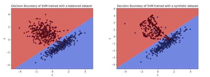

The left image shows the decision boundary of the original model, while the right one displays that of the SMOTE’d model. For starters, the hyperplane of the SMOTE’d model seems to favor the blue class, while the original SVM sides with the red class. I assume that the cause of this hyperplane shape is the lack of noisy red points among the blue cluster. 

Contrarily, the base dataset has several red points within the blue cluster, which might create a bit of bias on the model. The red region of the hyperplane is then pulled down since the model makes an effort to learn about those points. Thus, we can conclude that thanks to SMOTE, the algorithm was able to find a decision function that learned to separate our originally imbalanced dataset into two classes.

Recap and conclusion

At some point in your data science career, you are bound to encounter a situation in which you have to handle an imbalanced dataset. However frustrating, hopeless and rage-inducing this situation may be, techniques such as data oversampling and synthetic data generation allow us to make the best of the situation. 

In this article, I explained how to balance an imbalanced dataset using SMOTE, a data generator algorithm that adjusts the distribution of the classes in a dataset by creating data that resembles the original one. 

In the tutorial, we explored how the decision boundary of an SVM model evolves and reacts when fit with a balanced dataset, an imbalanced dataset, and a dataset enhanced by synthetic data produced with SMOTE. As a result, we obtained a model with a clear decision boundary that separated both classes.

This article was originally published at Kite‘s blog and republished here as part of content partnership program. Kite is a plugin for your IDE that uses machine learning to give you useful code completions for Python. Available for Atom, PyCharm, Sublime, VS Code, and Vim.